The current, gold-rush-era of NIL revenue sharing and the transfer portal has made it easier for more college football programs to “purchase” talent.
Alabama’s financial advantage in 2026 is that despite the rapidly changing economics of the game, Kalen DeBoer and the Crimson Tide do not have to rebuild their roster that way.
Now the on-field debate is almost the reverse of the financial one. Alabama is 8-2, yet the selection committee has Kalen DeBoer’s program at No. 3, ahead of unbeaten UCLA. The Tide’s win at Vanderbilt kept them moving, but the ranking criticism is not hard to understand: with two losses, how much should Alabama’s overall résumé outweigh a team that has not lost at all? That is a different question from what the roster is worth, and it makes this year’s Crimson Tide a useful case study in the gap between talent, spending and results.
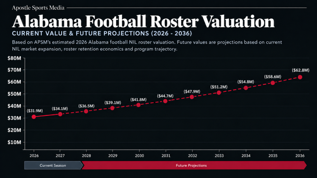
APSM currently places the Crimson Tide inside an estimated $31 million–$33 million open-market roster-value range, with a ~$31.9 million working midpoint.
Alabama ranks No. 13 nationally and No. 6 in the SEC in APSM’s current CFB roster valuation net reality model.
Approximately 59% of that value is tied to retained players, 22% to transfer additions and 19% to incoming recruits.
That composition matters more than the exact midpoint.
Alabama still uses the portal, but most of the roster’s value was recruited, developed and retained inside the program. The Crimson Tide are paying market prices where necessary without turning every offseason into a complete acquisition cycle.
The $31 million–$33 million range is intentional.
College-football player value now moves like a live market. Performance, injuries, role changes, commercial demand, portal leverage and broader NIL conditions can all move individual valuations during the season.
APSM therefore uses the range as the reader-facing valuation while the current ~$31.9 million midpoint remains the underlying snapshot for player-share calculations and other standardized math throughout this analysis.
That value should not be confused with Alabama’s disclosed football payroll. Direct university revenue sharing, legitimate third-party NIL, sponsorships, licensing and the much larger operating costs attached to coaches, facilities, recruiting, medical support and travel remain separate financial categories.
For the athletes themselves, gross roster value is only the beginning.
Alabama’s state tax environment, federal obligations, employment or self-employment treatment and representation costs determine how much of that earning power may eventually become usable capital.
Under APSM’s separate standardized $1 million tax-only benchmark, Alabama carries a Net Retention Score of 60/100.
The first APSM projection below begins with the current ~$31.9 million midpoint inside Alabama’s $31 million–$33 million 2026 roster range and applies the same illustrative 7% annual market-growth assumption used throughout the CFB roster series.
The current APSM valuation breaks Alabama’s roster into three major acquisition buckets:
- Retained players: ~$18.8 million | 59%
- Portal additions: ~$7.0 million | 22%
- 2026 recruits: ~$6.1 million | 19%
The balance is more important than any one percentage. Nearly three-fifths of Alabama’s current player value already existed inside the program, meaning Kalen DeBoer is not trying to replace the roster every offseason.
At the same time, the Tide carry meaningful value in both incoming recruits and portal additions, giving the program three different ways to acquire talent instead of relying almost entirely on one market. That matters because the economics of recruiting and the portal are different.
A transfer arrives with college film, production data and a clearer understanding of how he performs against collegiate competition. That generally reduces uncertainty, but proven talent can also demand more money immediately.
A high-school recruit arrives with more projection risk than a “veteran” player, but a program that identifies and develops that athlete before he becomes a premium college asset can potentially create substantial value internally (ROI).
Retention sits in the middle. Once Alabama turns a recruit into a productive player, the school still has to keep him. That has transformed development into an economic cycle:
recruit → develop → increase player value → retain → repeat → remain annual CFP contender
Alabama’s current roster is therefore less a transfer spending spree and more a portfolio constructed through multiple acquisition channels.
The current top five account for approximately $7.0 million, or about 21.9% of Alabama’s current ~$31.9 million working midpoint.
| Player | Pos. | Est. 2026 NIL Value | Share of Midpoint |
|---|---|---|---|
| Keelon Russell | QB | $2,000,000 | 6.3% |
| Ryan Coleman-Williams | WR | $1,800,000 | 5.6% |
| Jayvin James | OT | $1,150,000 | 3.6% |
| Jackson Lloyd | OT | $1,050,000 | 3.3% |
| Desmond Umeozulu | EDGE | $1,000,000 | 3.1% |
Keelon Russell is the financial centerpiece of Alabama’s 2026 roster. The sophomore QB currently carries an estimated value of approximately $2 million, making him the most valuable player on the Crimson Tide roster and one of the highest-valued quarterbacks in the SEC.
The interesting part is how quickly the market had to price him. Russell entered 2026 with limited college playing experience before winning the starting quarterback job.
Through Alabama’s early-season run, he has produced more than 1,100 passing yards, eight passing touchdowns and additional rushing production while completing roughly 71% of his attempts. Alabama lists him among the national leaders in several quarterback metrics.
Quarterback valuation can move faster than almost any other position because the athlete affects multiple financial variables simultaneously.
Production changes draft perception.
Winning increases national television exposure.
National exposure creates sponsorship inventory.
And a quarterback succeeding at Alabama carries commercial visibility few college programs can replicate.
Russell is therefore more than Alabama’s starting quarterback. He is the highest-value individual asset inside a $31.9 million roster.

Ryan Coleman-Williams sits just behind Russell at approximately $1.8 million. Unlike a quarterback valuation, wide-receiver economics generally depend more heavily on a combination of production, target share, explosive-play ability and commercial visibility.
Coleman-Williams already has all four. He entered 2026 as a preseason All-SEC selection and opened the year with 130 receiving yards against East Carolina, immediately reinforcing why his market value sits near the top of Alabama’s roster.
Williams was also selected to Nike’s 2026–27 Blue Ribbon Elite NIL roster, joining a group of Alabama athletes receiving direct access to one of the most recognizable sports brands in the world.
That is exactly why roster value and sponsorship income should not be treated as the same number.
The $1.8 million figure estimates his open-market player value. A Nike relationship exists inside a separate commercial layer that can increase the value of his name, image and likeness without automatically becoming part of a roster valuation.
Jayvin James is one of the best examples of why Alabama’s current roster cannot be explained purely through recruiting and retention.
James arrived after previous stops at Akron and Mississippi State and quickly earned Alabama’s starting right-tackle role.
He started every game to begin his Crimson Tide career after allowing only three sacks across 856 snaps at Mississippi State in 2025.
APSM currently values James at approximately $1.15 million, making him Alabama’s third-highest-valued player. That is a meaningful premium for an offensive lineman, but it makes sense financially.
Alabama has more than $2 million invested in the market value of Russell alone. Protecting that quarterback is not a secondary roster expense. It protects the value of the offense. James also represents Alabama’s portal strategy more clearly than a flashy quarterback acquisition would.
The Tide did not use the portal to completely replace their identity. They used it to acquire proven experience at a position where immediate reliability can protect several other assets at once.
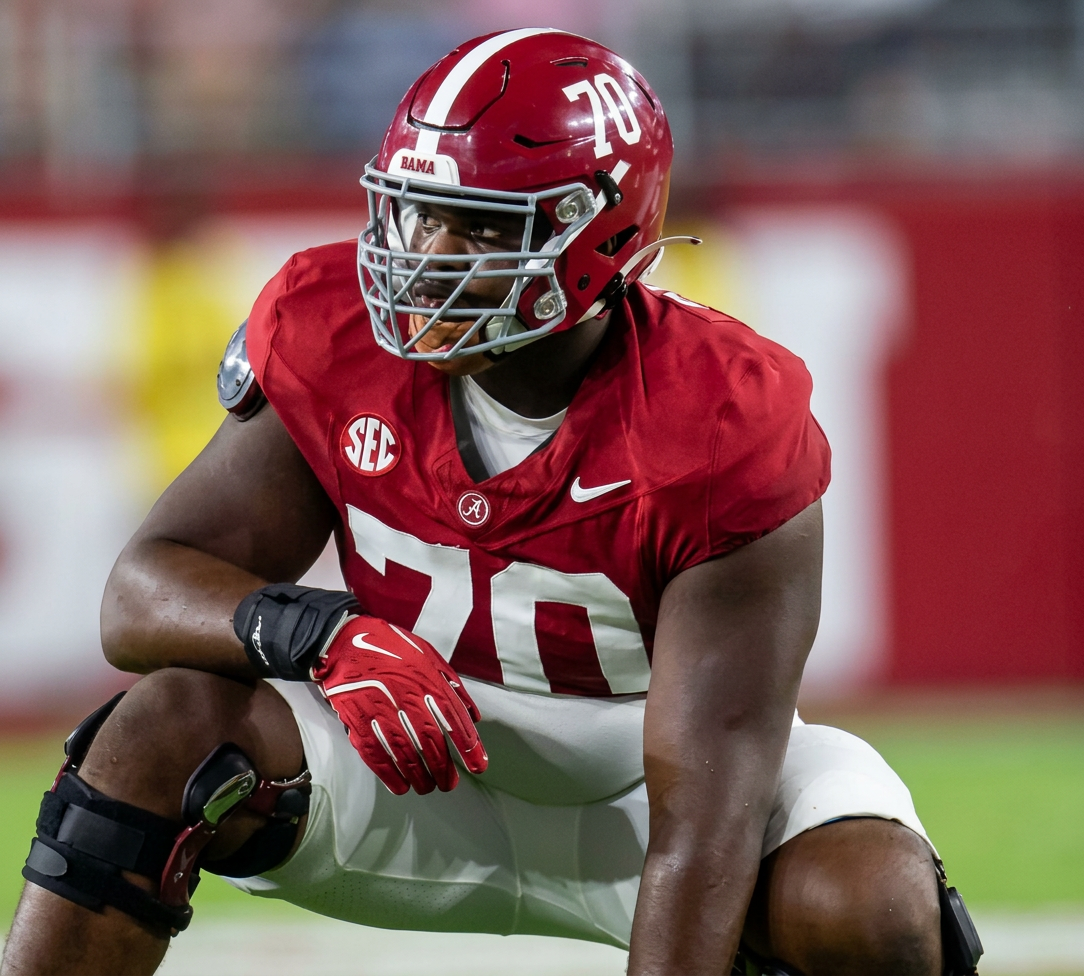
Jackson Lloyd carries an estimated value of approximately $1.05 million, putting a second offensive tackle inside Alabama’s top four.
That is not an accident.
When two offensive linemen sit near the top of a roster valuation, the money is telling us how the offense has been constructed.
Alabama’s most valuable individual player is a young quarterback. One of its most valuable skill-position players is a receiver.
Surrounding those two assets with premium offensive-line value reduces the risk that the entire offensive investment collapses because protection fails. Lloyd’s market value therefore carries a multiplier effect.
He is not simply worth what he produces individually. His position helps preserve the value of the players operating behind him.
Desmond Umeozulu rounds out Alabama’s current top five at approximately $1 million.
The senior transferred from South Carolina and entered Alabama as a pass-rush threat off the edge. He started early in the season before an injury interrupted his first year in Tuscaloosa.
His presence inside the top five illustrates another part of roster-market economics: premium positions get paid. Quarterbacks matter because they control the offense. Offensive tackles matter because they protect quarterbacks. Edge defenders matter because they destroy that protection.
A seven-figure valuation at edge therefore fits the same roster logic as Alabama placing two offensive tackles near the top of its financial hierarchy.

The 2026–27 school revenue-sharing cap is approximately $21.58 million per participating institution.
That figure increased from the original $20.5 million first-year limit and represents the maximum schoolwide amount participating institutions may distribute directly to athletes under the current House settlement structure.
It should not be added directly to Alabama’s ~$31 million – $33 million roster valuation and described as a fictional ~$53.5 million football payroll.
They measure different things.
- $31 million–$33 million is APSM’s current estimated Alabama football player market-value range.
- ~$31.9 million is APSM’s current working midpoint.
- $21.58 million is the schoolwide institutional revenue-sharing ceiling across all sports at a university.
Third-party NIL exists separately from both. That distinction is exactly why headline spending estimates can become misleading.
A university can allocate enormous amounts of capital toward athlete compensation without every dollar being attributable specifically to Alabama football players.
Alabama Athletics reported approximately $267.4 million in total FY2025 revenue against roughly $234.7 million in expenses, producing an operating surplus of roughly $32.7 million.
Football alone generated ~$147.7 million in operating revenue.
That is why “Alabama has hundreds of millions of dollars” and “Alabama has a $31.9 million roster” are not contradictory statements. The athletic department is the business. The football roster is one collection of assets inside that business.
Football revenue must help cover coaching compensation, scholarships, recruiting, travel, facilities, support staff, nutrition, equipment, medical services, administration and dozens of other costs before anyone can pretend total revenue equals player compensation.
That difference is basic accounting. Revenue is not profit. Program spending is not player value.
Roster valuation is not net income.
Want to calculate your own net reality?
Use the –> APSM Net Income Calculator
Alabama’s athletes also operate inside a commercial system that extends beyond direct university payments. The school continues to work with dedicated NIL infrastructure and brand partners, while Nike’s 2026–27 Blue Ribbon Elite program added 18 Alabama athletes, including several football players such as Russell, Coleman-Williams and Yhonzae Pierre.
That matters because athlete value is no longer generated solely by football production.
An athlete can monetize:
- sponsorships
- licensing
- content
- merchandise
- appearances
- camps
- digital media
- social audiences
- business partnerships
A roster valuation is therefore only one side of the athlete’s financial life. The other side is what the athlete does with the commercial attention created by playing at Alabama.
Alabama’s investment in football does not stop with athletes. The university extended Kalen DeBoer through January 2033 in April 2026, adding two years to his agreement. The revised contract keeps him in Tuscaloosa through the 2032 season.
Reported terms put the agreement at roughly $87.5 million over seven years, or approximately $12.5 million annually (base salary).
That money should not be included in Alabama’s $31 million – $33 million roster valuation. It does, however, provide useful context.
Alabama is effectively paying eight figures annually for the executive responsible for managing a player asset base valued at nearly $32 million, while the football operation itself generates close to $148 million in annual operating revenue.
That is not amateur economics. It is a large sports enterprise operating inside a university.
Using the same standardized 2026 framework APSM applies elsewhere, DeBoer’s contract also provides a useful gross-to-net example.
If his full ~$12.5 million annual base compensation were modeled as W-2 income for a single filer, APSM estimates approximately ~$7.2 million could remain after federal income tax, employee Social Security and Medicare taxes and Alabama state income tax; before incentives, itemized deductions, benefits, retirement contributions or individualized tax planning.
That represents roughly 58% of gross compensation under the standardized illustration. The comparison is important because a $12.5 million coaching contract and a $12.5 million bank balance are two completely different financial numbers.
APSM estimate only: DeBoer’s actual filing status, deductions, benefits, contract structure and tax return are private. The example is designed to illustrate the financial mechanics of a coaching contract, not estimate his private tax liability.
For the federal baseline, the 2026 single standard deduction is $16,100, the 37% bracket begins above $640,600 of taxable income, and the 2026 Social Security wage base is $184,500.
Alabama’s state income-tax system looks straightforward on the surface. It is not. The state uses graduated individual rates of 2%, 4% and 5%, with the 5% tax bracket beginning at relatively low taxable-income levels.
For seven-figure NIL earners, the headline marginal state rate is effectively 5%. But, Alabama has an unusual feature that materially affects the calculation: federal taxes paid can be deducted when calculating Alabama taxable income.
That means simply multiplying a $2 million NIL valuation by 5% would overstate the athlete’s actual Alabama income-tax liability. Federal income tax remains the largest component for a high earner.
Applicable self-employment or employment taxes may also apply depending on how the income is structured. Representation costs reduce usable capital.
Athletes earning money across multiple states may create additional filing obligations.
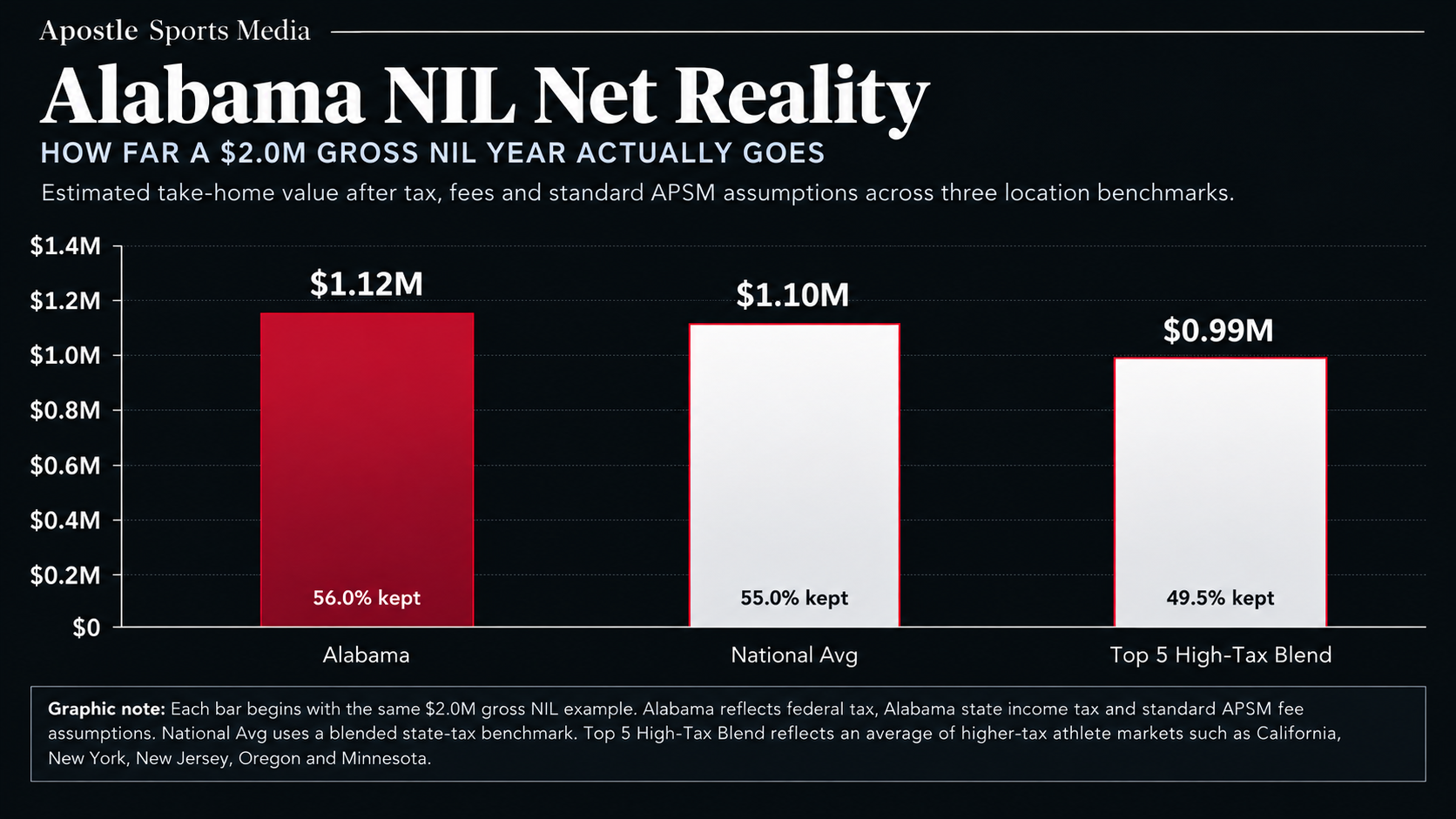
The easiest way to understand Alabama’s financial position is therefore to keep the athlete’s gross income constant and change only the location.
For more information on how income tax drag actually affects collegiate athletes’ net reality Read Our –> State Income Tax Explained for NIL & Professional Athletes – The States That Cost the Most
Alabama’s relatively manageable income-tax structure does not mean the entire tax system is light. The state imposes a 4% general sales tax, while local taxes push the average combined state-and-local sales-tax rate to approximately 9.46%, one of the highest averages in the country.
That matters differently from income tax. Income tax affects what an athlete retains when money is earned. Sales tax affects what happens when retained income is spent.
An athlete earning $2 million can preserve meaningful capital through good tax planning and then still burn through it quickly by consuming aggressively. Cars, clothing, electronics, entertainment and other taxable purchases turn after-tax income into additional tax payments.
That is why earning power and purchasing discipline are separate financial skills.
For more information on Alabama state taxes, cost of living metrics and real estate markets head to the APSM State Athlete Tax Glossary –>
Alabama State Athlete Taxes
Alabama moves in the opposite direction on residential property taxes.
The state’s effective property-tax rate on owner-occupied housing is approximately 0.37%, among the lowest in the country.
At that statewide effective rate, a hypothetical $1 million owner-occupied property represents roughly $3,700 per year in property tax before local variation and individual assessment differences.
That does not make homeownership free.
Insurance, repairs, utilities, maintenance and transaction costs still exist.
For an athlete considering long-term ownership, Alabama’s property-tax environment can reduce one of the carrying costs attached to real estate.
Tuscaloosa also gives Alabama athletes a relatively low housing-cost base compared with many major sports markets.
As of August 2026, Zillow placed the average Tuscaloosa home value at approximately $245,668, up about 0.9% year-over-year, while average rent was approximately $1,448 per month.
The national typical home value was roughly $368,697 during the same period. That difference matters when a college athlete suddenly begins earning six or seven figures.
A $1 million income in Tuscaloosa does not require the same housing commitment as a $1 million income in Los Angeles, New York or Miami.
The lower housing baseline can leave more capital available for reserves, investments or future opportunities. Again, geography affects wealth through more than one tax rate.
Income tax affects earnings.
Sales tax affects consumption.
Property tax affects ownership.
Housing prices determine how much capital has to be committed to the asset in the first place.
Because private contracts, tax returns and representation agreements are not publicly available, APSM cannot determine the exact take-home income of Alabama’s players from market valuations alone.
Instead, APSM applies the same standardized Net Reality framework used throughout these roster valuations.
For the Alabama model, APSM accounts for:
- applicable federal taxation
- Alabama’s state-income-tax structure
- the state deduction for federal income taxes paid
- employment or self-employment/FICA treatment where applicable
- a standard 3% contract-negotiation and representation estimate
- 0% personalized expenses
Personal expenses are intentionally excluded from the standardized article model.
One athlete might spend $30,000 running his business. Another might spend $250,000 across housing, training, travel, family support and lifestyle. Those variables belong inside the APSM Net Income Calculator, not inside a standardized roster article where they would have to be invented.
Using the standardized framework, APSM models approximately 56% retained capital for the high-income Alabama example. That does not mean every Alabama athlete keeps exactly 56 cents of every dollar.
It gives APSM one consistent baseline for comparing athletes, schools and states without changing the methodology every time the uniform changes.
This is different from the APSM Net Retention Score, which uses a standardized $1 million tax-only benchmark with no representation fees or personalized expenses.
Alabama scores 60/100 under that standardized benchmark.
The roughly 56% player-retention example above uses a $2 million gross amount and includes the 3% representation assumption, which is why the two figures should not be treated as interchangeable.
That distinction is intentional: the Net Retention Score compares jurisdictions, while the player-level Net Reality model estimates how taxes, fees and income structure can affect an individual earning scenario.
Applied to Alabama’s five highest-valued players, ~$7.00 million in combined roster value translates to roughly $3.85 million in modeled retained capital.
Those figures are not reported salaries or private tax outcomes. They show the difference between headline player value and potentially usable capital.
| Player | Gross Valuation | Illustrative Deductions | Illustrative Net Capital |
|---|---|---|---|
| Keelon Russell | $2,000,000 | ~$890,000 | ~$1,110,000 |
| Ryan Coleman-Williams | $1,800,000 | ~$810,000 | ~$990,000 |
| Jayvin James | $1,150,000 | ~$520,000 | ~$630,000 |
| Jackson Lloyd | $1,050,000 | ~$480,000 | ~$570,000 |
| Desmond Umeozulu | $1,000,000 | ~$450,000 | ~$550,000 |
The most valuable financial advantage available to a high-earning college athlete may not be the amount earned.
It may be the age at which the money arrives.
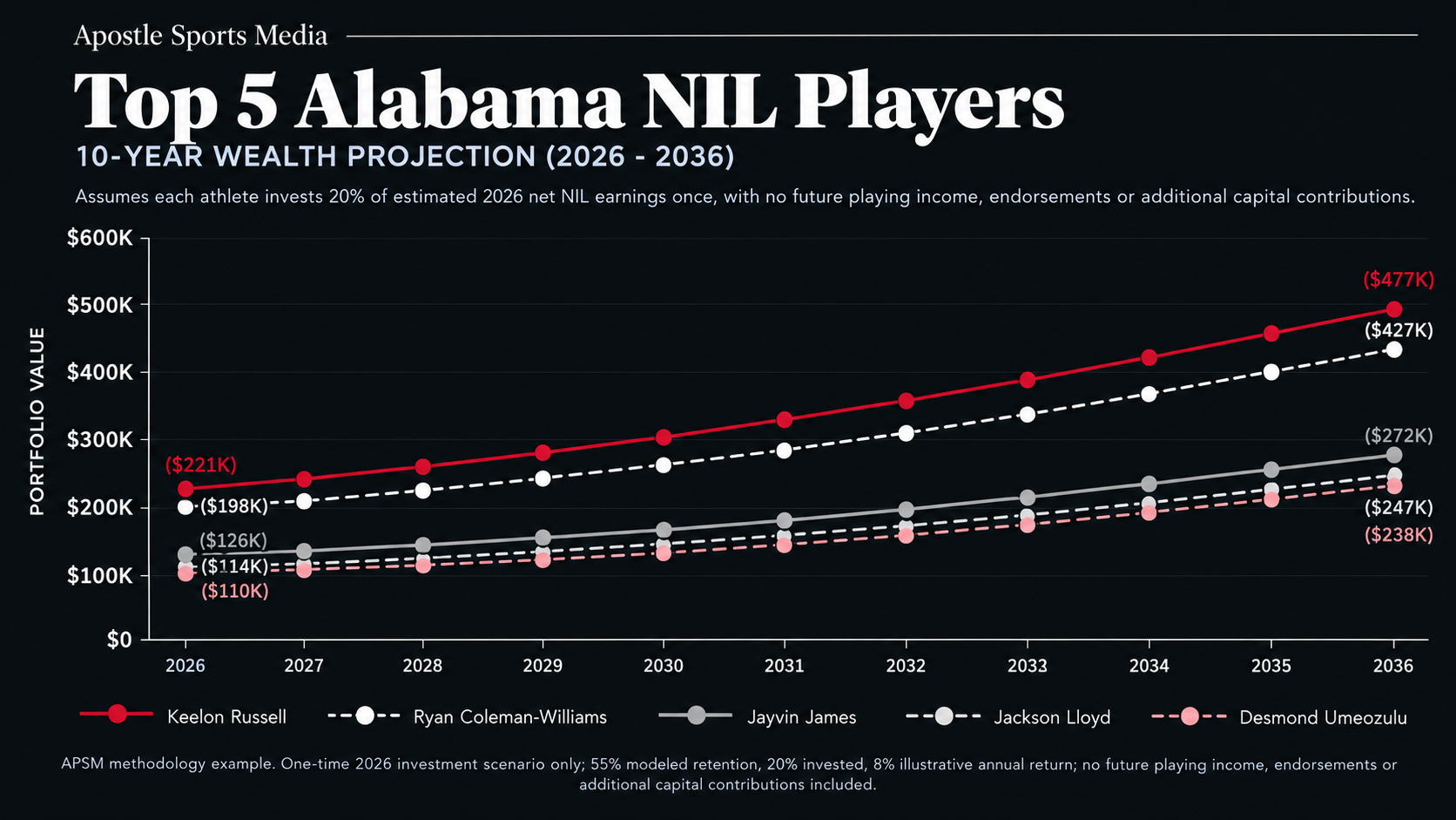
Using the standardized model above, Russell’s ~$2.0 million valuation corresponds to approximately $1.11 million in retained capital.
If he invested only 20% of that modeled net amount once, approximately $221,000 would enter productive assets immediately.
No future NIL contribution is required for that first investment to keep working. At an illustrative 8% annual return, the original $221,000 could grow to approximately $478,000 over 10 years.
That does not require a future NFL contract. It does not require another sponsorship. It does not require another dollar to be contributed.
It only requires the original capital to survive long enough to compound.
Tuscaloosa Real Estate
Real estate creates another option. With Tuscaloosa’s average home value around $246,000, a seven-figure athlete could potentially purchase substantial home equity without committing the majority of his available capital to housing.
That does not automatically make buying a property the right decision. The athlete still has to consider financing, liquidity, transaction costs, maintenance, insurance, investment horizon and whether the property is being purchased as a residence or an actual investment.
The important advantage is optionality. High income in a relatively low-cost housing market gives the athlete more choices.
The cleanest way to measure the long-term value of Alabama’s current NIL market is to remove future success from the equation entirely.
Assume the current 2026 season is the only major football income these players ever receive.
- No future Alabama NIL payments.
- No additional endorsements.
- No NFL contract.
- No additional investment contributions.
Under the standardized APSM model, Alabama’s five highest-valued players invest 20% of their modeled 2026 retained capital in a standard index fund or mutual fund once; then allow that money to compound at an illustrative 8% annual return through 2036.
That creates a much more disciplined financial exercise than assuming today’s valuation continues year after year.
It answers a simpler question: What can one major college earning window accomplish by itself?
The graphic below uses only the capital generated from the 2026 season. Everything after that comes from compounding.
Why This Data Matters
The projection is not designed to predict Russell, Coleman-Williams or James’ future net worth.
Their real careers may look completely different. The purpose is to measure the value of the starting point. A college athlete who reaches professional football with hundreds of thousands of dollars already invested enters the NFL in a fundamentally different financial position from an athlete beginning with no productive assets.
The rookie contract no longer has to become the beginning of wealth creation. It can become another contribution to wealth that already exists. And for athletes who never reach the NFL, the lesson may be even more important; Temporary athletic income can still create permanent capital.
Alabama’s broader financial position becomes easier to compare once the player-specific calculations are separated from APSM’s standardized Net Retention Score.
Under the APSM benchmark, every state begins with the same $1 million of gross athlete income.
Agent fees and personalized career expenses are removed from the comparison so the score isolates the underlying tax environment rather than the athlete’s individual representation or spending decisions.
For Alabama, that produces an APSM Net Retention Score of 60/100.
That score should not be confused with the roughly 56% retention modeled at the standardized $2 million Alabama player example above.
The player model includes additional assumptions such as representation and evaluates a different gross-income level.
The Net Retention Score intentionally removes agent fees and individualized expenses and fixes gross income at $1 million so Alabama can be compared directly with Texas, California, Florida, Georgia or any other jurisdiction under the same tax-only benchmark.
Alabama’s 5% top marginal state income-tax rate creates more drag than a no-income-tax jurisdiction such as Texas, but the state’s deduction for federal income taxes paid softens part of that burden for higher earners.
That is why Alabama can still produce a relatively competitive 60/100 retention score without being a zero-income-tax state.
The score is not a prediction that every Alabama athlete literally keeps 60 cents of every dollar. It is the standardized state-level baseline underneath the larger Net Reality calculation.
APSM Net Retention Score: Alabama – 60/100

APSM FINANCIAL REPORT · $9.99
The Million-Dollar Illusion
A million dollars earned is not a million dollars kept. Explore the taxes, fees and financial decisions behind the headline.
36-page research report · Two fillable worksheets included
For Athletes
Alabama’s 60/100 APSM Net Retention Score gives athletes a relatively competitive tax-only starting point, but gross value still has to survive federal taxes, income structure, representation and individual financial decisions before it becomes lasting capital.
Alabama shows why financial literacy has become part of athlete development. A seven-figure roster valuation creates opportunity, but the athlete still has to navigate taxes, contract fees, multi-state income, spending and investment decisions before the money can become wealth.
For Agents
The current Alabama roster also shows that representation is no longer simply about negotiating one sponsorship.
Agents increasingly operate across direct institutional compensation, third-party NIL, transfer-market leverage, commercial partnerships and eventually professional contracts.
For Sponsors
Alabama offers a rare combination of national football exposure and increasingly organized athlete-brand infrastructure.
Nike’s Blue Ribbon Elite program demonstrates what happens when a major brand can access athletes who already perform inside one of the most recognizable sports brands in America.
For Alabama
The university’s challenge is allocation. Alabama must fund direct revenue sharing, retain valuable players, acquire transfers, recruit elite high-school talent, pay an eight-figure head coach and operate a football program generating nearly $148 million in annual revenue without pretending all of those dollars belong to the same accounting bucket.
Alabama currently sits inside APSM’s estimated $31 million – $33 million 2026 football roster-value range, with the current player-level dataset centered around a ~$31.9 million working midpoint.
Roughly 59% of that value belongs to retained players, 22% to portal additions and 19% to recruits.
The Crimson Tide still spend in the transfer portal. They still recruit against the wealthiest programs in the country. They still operate inside the new revenue-sharing system and a growing third-party NIL economy.
But most of Alabama’s roster value was not purchased in one offseason.
It was recruited, developed and retained.
Around that player portfolio sits a much larger enterprise: roughly $267 million in annual athletics revenue, nearly $148 million in football revenue, an eight-figure head-coaching contract and a commercial ecosystem capable of connecting Alabama athletes with national brands.
For the athlete, Alabama also carries an APSM Net Retention Score of 60/100 under the standardized $1 million tax-only benchmark.
That is a solid starting point. It is not the finish line.
A $2 million roster valuation is not $2 million of wealth. Gross income still has to survive taxes and fees. Retained income still has to survive lifestyle and bad decisions. Whatever remains then has to become savings, investments, business equity, real estate or another productive asset before temporary earning power becomes lasting financial security.
That is the Net Reality.
APSM currently places Alabama’s 2026 football roster in an estimated $31 million–$33 million open-market range, with a current working midpoint of approximately $31.9 million. The range reflects the fact that college football player values can move during the season as performance, injuries, portal activity and commercial demand change.
Alabama’s five highest-valued players combine for approximately $7.0 million, equal to roughly 21.9% of APSM’s current ~$31.9 million midpoint.
Keelon Russell (QB): ~$2.0M
Ryan Coleman-Williams (WR): ~$1.8M
Jayvin James (OT): ~$1.15M
Jackson Lloyd (OT): ~$1.05M
Desmond Umeozulu (EDGE): ~$1.0M
The distribution is notable because Alabama’s highest-value capital is spread across quarterback, receiver, offensive tackle and edge rather than being concentrated entirely in one superstar.
No. The $31 million – $33 million range represents APSM’s estimate of Alabama football’s open-market player value, not a disclosed university payroll. Direct institutional revenue sharing, legitimate third-party NIL, sponsorship income and broader football operating expenses are separate financial categories.
Using APSM’s standardized 2026 framework with progressive federal taxation, applicable employment or self-employment/FICA treatment, Alabama’s state-income-tax structure, a 3% representation estimate and 0% personalized expenses, the $2 million benchmark models approximately $1.12 million of retained capital, or roughly 56% of gross.
Actual results can vary substantially based on income structure, filing status, deductions, residency and individual circumstances.
Alabama uses graduated individual income-tax rates of 2%, 4% and 5%, with high earners generally reaching the 5% marginal rate.
Alabama also allows federal income taxes paid to reduce Alabama taxable income, which makes the effective burden more nuanced than simply multiplying gross athlete income by 5%.
Under APSM’s standardized $1 million tax-only benchmark, Alabama produces a Net Retention Score of 60/100.
- Georgia 2026 CFB Roster Valuation: Net Reality
- Ole Miss 2026 CFB Roster Valuation: Net Reality
- Texas 2026 CFB Roster Valuation: Net Reality
- Ohio State 2026 CFB Roster Valuation: Net Reality
- Alabama Athlete Taxes
Sources & Methodology
APSM’s Alabama roster valuation is an independent analytical estimate based on published roster information, reported athlete-market evidence and APSM’s player-level financial modeling.
APSM treats third-party valuations as inputs, not verified compensation or a disclosed university payroll.
- Roster documentation: The official 2026 roster establishes program and player context, not the price of every private NIL agreement.
APSM valuation and Net Reality methodology: APSM keeps estimated player market value, institutional operating expenditure, reported compensation and after-tax retained capital separate. All financial midpoints, player allocation shares, tax assumptions, retention benchmarks and investment scenarios already in this article remain unchanged. For APSM’s standard method, see the Net Income Calculator and Net Reality methodology.
Disclaimer: This article contains general financial information for educational purposes and does not constitute professional advice. APSM estimates are derived from publicly available information, tax assumptions, finance modeling, and industry-standard fee structures. Actual earnings may vary based on residency elections, private contract provisions, image/media rights agreements, bonuses, and tax filings.